Example 7: Three-line section from C and L matrices
Netlist: examples/three-line-CL.cir
Goal: use the general C/L input, which is what a 2-D field solver gives you, for an inhomogeneous three-conductor section. Then read the modal analysis and build a symmetric coupler with the centre line as input.
The matrices come from comb-over's field solver (manual §4.3) for three 0.8 mm microstrip lines with 0.15 mm gaps on 0.508 mm RO4350B (εr 3.66) with 1 oz (34.79 µm) copper:
node solver/cli.mjs --W 0.8,0.8,0.8 --S 0.15 --h 0.508 --er 3.66 --t 0.03479
Input
cline TL3
  C [103.32058p -24.996611p -1.0254662p; -24.996611p 113.18589p -24.996611p; -1.0254662p -24.996611p 103.32058p]   # F/m (Maxwell matrix)
  L [308.1564n 103.46107n 43.654707n; 103.46107n 294.99833n 103.46107n; 43.654707n 103.46107n 308.1564n]   # H/m
  len 90deg
  A l_cpl c_in  r_cpl
  B l_iso c_out r_iso
end
Requirements on the matrices:
- C is the Maxwell matrix. The diagonal is each line's total capacitance with the others grounded; the off-diagonals are negative. If your solver reports ground and mutual capacitances instead, convert with Cii = Cgi + ΣCmij and Cij = −Cmij.
- L is the inductance matrix. All entries are positive.
- Both are symmetric, and C must be positive definite.
The tool checks all three.
The modal analysis
The Line sections panel shows:
| mode | εeff | Zmode (Ω) | voltage vector (lines 1, 2, 3) |
|---|---|---|---|
| 1 | 3.0589 | 80.88 | [0.557 0.615 0.557] |
| 2 | 2.4805 | 50.35 | [0.707 0 −0.707] |
| 3 | 2.2468 | 34.99 | [−0.409 0.816 −0.409] |
How to read it:
- Number of modes. Three conductors give three quasi-TEM modes with three different velocities, which is the hallmark of an inhomogeneous medium.
- Mode 1 is the all-in-phase "even" mode. It has the most field in the substrate, so the highest εeff, and the highest impedance.
- Mode 2 is the antisymmetric outer-line mode. The centre line carries no voltage, because by symmetry it cannot couple to this mode.
- Mode 3 drives the centre line against the outer lines.
len 90deg is referenced to the mean of √εeff over the three modes, which gives 15.54 mm at 3 GHz. Each mode therefore sees a slightly different electrical length.
The characteristic admittance matrix Yc = W diag(v) Wᵀ (§9 of the manual) is, in mS,
[ 19.473  −5.689  −0.389 ]
[ −5.689  21.946  −5.689 ]
[ −0.389  −5.689  19.473 ]
Note the small but non-zero coupling between the outer lines (−0.389 mS). The Cg/Cm nearest-neighbour model in the filter examples ignores this kind of term unless you add it with Cm(1,3).
The coupler
Port 1 drives the centre line at end A. Port 2 is the centre line's other end. Ports 3/5 are the outer lines at the input end (coupled), and ports 4/6 are the outer lines at the far end (isolated).
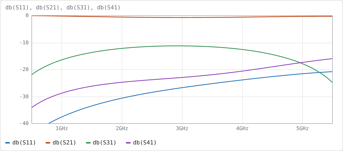
| f (GHz) | S11 | S21 | S31 = S51 | S41 = S61 | total coupled (S31 + S51 power) |
|---|---|---|---|---|---|
| 1.5 | −33.56 | −0.41 | −13.73 | −26.23 | −10.72 dB |
| 3.0 | −26.79 | −0.76 | −11.27 | −22.99 | −8.26 dB |
| 4.5 | −22.67 | −0.47 | −14.46 | −19.05 | −11.45 dB |
- Symmetry.
db(S31/S51)is zero to 2e−13 dB, because the structure is symmetric and the centre line feeds both outer lines equally. - Directivity. It is only about 12 dB at f0, the same inhomogeneous-medium problem as in Example 2. Lumped compensation capacitors between the lines at each end would improve it.
- Match. S11 ≈ −27 dB at f0. The widths were picked from a coarse search for a match better than −20 dB with about −9 dB total coupling; they were not optimised.
The same section from its geometry
The section can also be given by its geometry. The field solver then runs inside comb-over:
.substrate jlc-ro4350b-0.508
cline TL3
  geom msl
  W [0.8mm 0.8mm 0.8mm]
  S 0.15mm
  len 90deg
  A l_cpl c_in  r_cpl
  B l_iso c_out r_iso
end
This gives the same matrices: the substrate preset carries the copper thickness, so the solver gets the same rectangular strips. The geometry form also adds conductor and dielectric loss. At 3 GHz the modal Q is 168 for the in-phase mode, 127 for the outer-line mode and 102 for the centre-against-outer mode, which crowds current into both gaps. S21 goes from −0.76 dB to −0.82 dB.
Try
- Change the widths in the geometry form, for example
W [0.8mm 1.0mm 0.8mm], and watch the match and the coupling change. The centre-line width sets the input impedance. - Multiply every entry of C by 1.2 and divide every entry of L by 1.2. The εeff values are unchanged and every Zmode drops by 1.2. Watch S11 change.
- Set L = μ0ε0·C0⁻¹ for some air-filled C0 to make your own physically consistent pair. A field solver gives you C and C0 (C with the dielectric removed), and L follows exactly that way.
- Replace the end connections to make a three-line comb or interdigital resonator array. For example,
A 0 0 0andB r1 r2 r3with loading capacitors gives an inhomogeneous comb-line, which the synthesiser does not yet cover.